I’ve been mulling over the accuracies of my little 24-bit digital acquisition unit and have finally convinced myself that it’s working properly (a discussion worthy of its own post). So, now I’ve gotten to the point where it’s appropriate to characterize the sensors that I’ll be using along with the DAQ to make sure that they have the bandwidth that my learning algorithms may eventually need.
Luckily, the IEEE has been getting papers on things like this for many, many years, and finding literature upon which to base my analysis was very easy. I found ‘Frequency response of Measurement Current Transformers’ by A. Cataliotti Et. Al. to be particularly interesting, but was dissappointed to find that their methods of determining frequency responses of current transformers made no mention of the hardware required for the current source used in their paper. Based off of the figures in their paper, and the methodology behind their analysis, I assumed that they were using some sort of resistive load with an alternating excitation current. Most likely an inverter with a frequency sweep, which would give a bode plot of frequency, magnitude, and phase when plotted on a loglog scale.
As I wasn’t about to build my own inverter in a Sunday afternoon, I wanted to see if I could hack something together which would still get the job done. Square waves are easy, and the perfect square wave is not bandwidth limited, which is to say that it can be represented by an infinite sum of scaled and shifted sine waves of various frequencies, and has a known pattern to the amount of power stored in its harmonics. Great, I’ll just excite the current transformer with a square wave, center the square wave frequency close to where I think the cut-off might be, and find when the harmonics start to roll-off faster than they should. Simple, right? Well, it’s a little more complicated than that, as creating that sharp edge on a square wave that contains all that spectral energy can actually be pretty difficult. I’ll touch upon this further a little later in this post.
To get that square wave into the system, I needed a way of amplifying a reference signal from a signal generator. In poking around my spare parts, I found a beefy FDB86135 MOSFET and borrowed a si8233 from someone in lab to drive it. While the signal generator is technically capable of driving the gate of my FET on its own, the gate charge of 116 nanoColoumbs meant that if I wanted to drive the circuit past 20kHz, that I’d really need to use a driver, hence the si8233.
For the load I took the old 4.5 Ohm resistor pack I soldered up for use with the autotransformer and repurposed it as the excitation load. Before repurposing it, it was a really, really dangerous thing to be left unattended. I caught someone thinking about plugging it into the unregulated 120 VRMS wall-juice in an attempt to turn it into a cloud of smoke.
Before this, I had completely underestimated the usefulness of a fat resistor and a variable AC load. Anyway, moving on…
I used some reference parts in eagle, made a quick layout, saved the gerbers to a thumbdrive and went down to the ProtoMat to cut it out. As always, you must respect the LPKF’s Warmingtime. It’s a proper noun.
Using the 16mil double-flute end mill has always given me great results.
All assembled! So simple!
Now, the square wave that’s going to sink current through the mosfet and excite the load isn’t going to be purely a square wave. Since there’s input, output, and reverse transfer capacitance; and resistance in the wires, load, and Rds_on of the FET, there’s going to be some sort of a RC time constant of the circuit itself which smooths out the rising edge. Additionally, there is a finite time where the MOSFET goes through a linear region as the voltage on the gate rises from zero up to the full saturation voltage. In this case a 4.7 Ohm resistor was added to stop ringing from occuring on the gate line, which exaggerates that even further. All of these contribute to a more round rising and falling edge of our square wave and a less rich excitation. However, in the case of this system, the effective bandwidth limitation of the excitation circuit is negligible, as the magnetics of the current transformer will attenuate much more high-frequency energy.
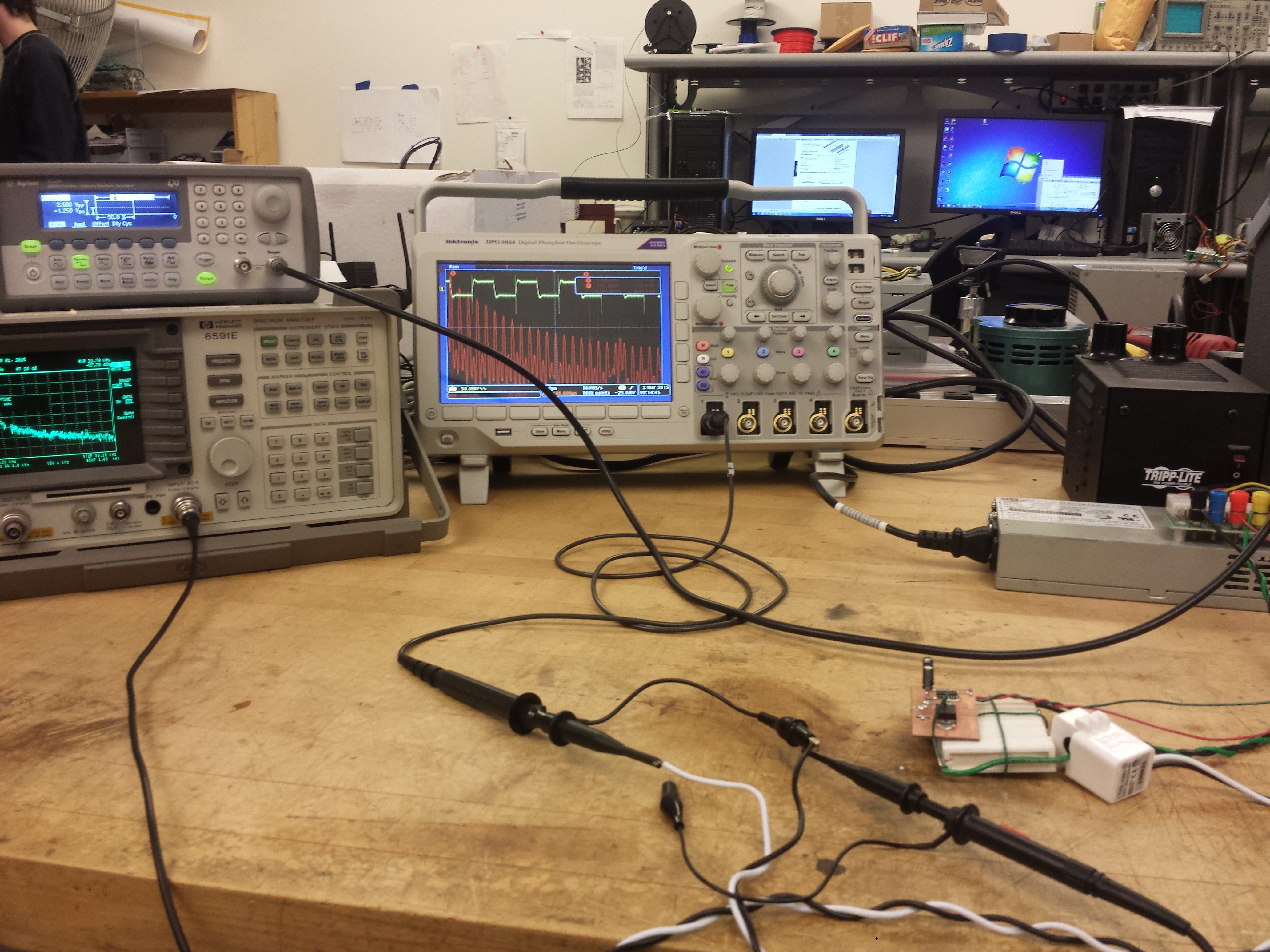
Here’s a view of the test setup, for power I’m using one of my more low-impedance-path-explodey-friendly 1-U ATX supplies with my ATX breakout on it:
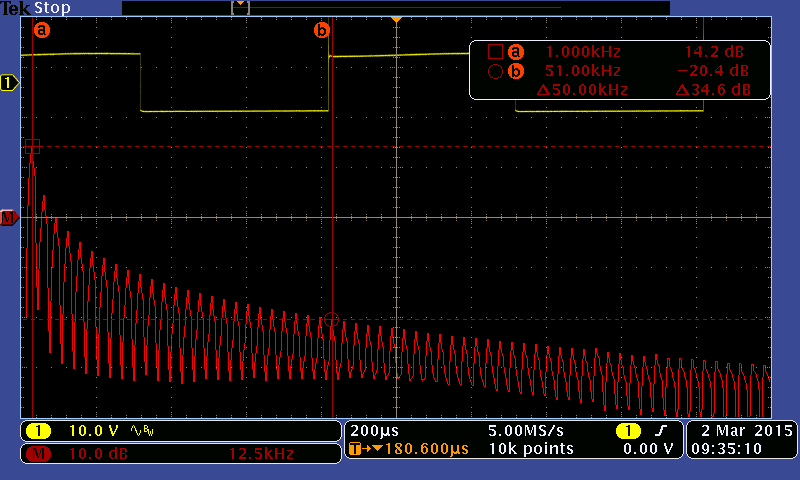
The first test is to see what the PSD of the excited load looks like. Call this Fig. 1
Now let’s look at how that signal looks through the CT. Hey, I just realized that the oscope has its time and date settings off by 24 hours… Call this Fig. 2
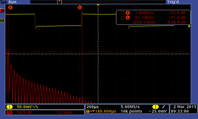
There’s a lot of ways to interpret these results, but, let me walk you through what’s most important to my application here. One of the first things that you can ignore immediately is the shift in magnitude of the entire PSD. This is to be expected, and if you’re eagle-eyed you’ll have already noticed that the voltage/div of channel 1 is way larger in Fig. 1 than it is in Fig. 2, which explains the big difference in the sum total energy in the PSD. If I had cared to figure out how to normalize stuff in the math menu of the o-scope that wouldn’t have shown up.
The biggest thing to note is that from the fundamental 1kHz tone to the harmonic at 51-kHz that there’s a 35dB change in power for, what I’m going to call, the full-bandwidth excitation signal. Note that as we go through the current transformer in Fig. 2 that the PSD starts to roll of faster at 51-kHz, and that the edges of the sampled square wave. You’ll see that the PSD starts to attenuate by ~3dB at 51-kHz through the CT, which would imply that the CT has a frequency bandwidth well within the requirements of my system (~16kHz). Given that my DAQ has ~96dB of dynamic range, I thought that it would be interesting to compare these results to what my DAQ reads.
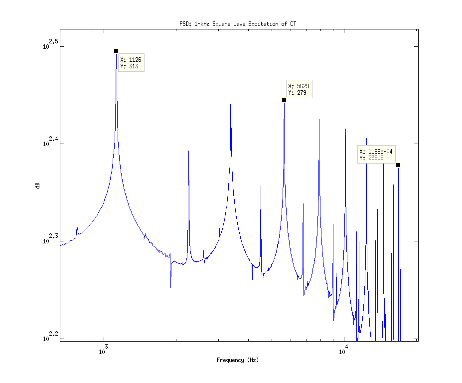
Note that the oscilloscope had a resolution of 12.5kHz/div while this DAQ has an anti-aliasing filter on it which starts to roll off at 3dB at ~8kHz. Also note that I was riding dirty with the signal generator and bumped up the frequency past 1kHz for this test, but was too lazy to go back and redo it to center the fundamental tone at 1kHz.
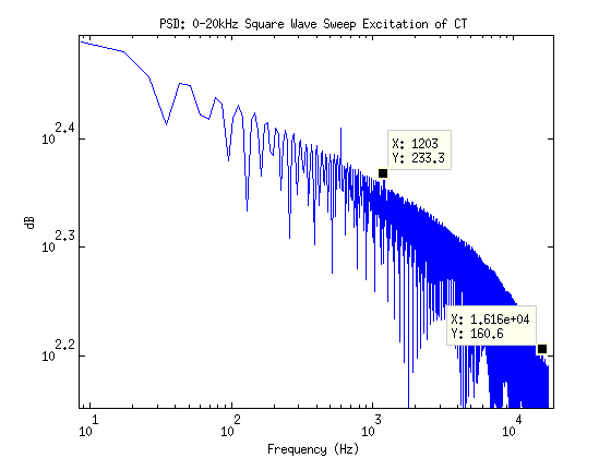
I wonder what a sweep from 1-kHz to 20-kHz will look like with a datarate of 32kSpS?
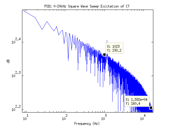
Let’s bump that waaaay up and max out the mcp3912
Cool! At this temporal resolution you can actually see the equiripple of the 3rd order digital sinc filter due to its settling time. (Delta-Sigma 4 lyfe)
Not bad for a 3 hour push on a Sunday afternoon!