Contents
clc
%clear all
close all
System ID
Here I take a bandwidth limited white-noise input, excite a system with it, use arx to build a model of the input/output.
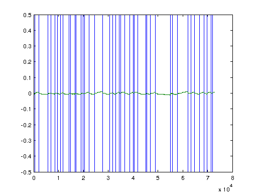
%load strain
Ts = 1/1000; % Time-step
na = 3; %order denominator model
nb = 3; %order numerator model
nc = 2; %order numerator noise model (BJ and ARMAX)
nd = 2; %order denominator noise model (BJ)

output1 = output(8100:8.1*10^4,:);

U = output1(:,3);
U1 = output1(:,2);
Y = output1(:,1);
N = length(U);

% U = U(8100:(8.2*10^4));
% U1 = U1(8100:(8.2*10^4));
% Y = Y(8100:(8.2*10^4));

% Remove nans if they exist.
unan=isnan(U);
ynan=isnan(Y);
for i=1:length(U)
    if (unan(i))
        U(i) = U(i-1);
    end
    if (ynan(i))
        Y(i) = Y(i-1);
    end
end
unan=isnan(U);
ynan=isnan(Y);
figure;
plot([unan ynan]);

% Linearizing data, if needed.
K = 0;
V = (U -0*K*(U.^3).*(Y));
Y = (2*3.14/2048)*Y;

plot([V,Y])
Estimate models using various system ID methods.
highorder = 100;
data=iddata(Y,U1,Ts);
data1=iddata(Y,U,Ts);
data = [data, data1];
data = data(:,1,:) %keep only one of the outputs MISO
nk = delayest(data1);
modelARX = arx(data, [highorder [highorder highorder] [nk nk]]);
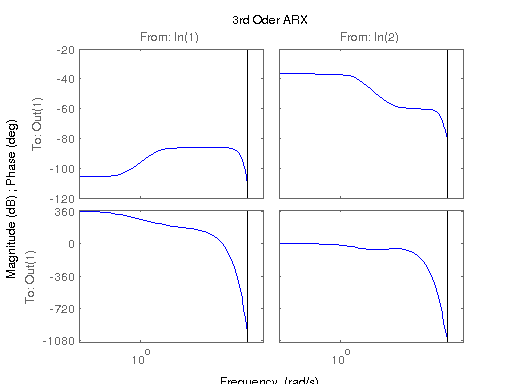
modelARX3 = arx(data, [3 [3 3] [nk nk]]);
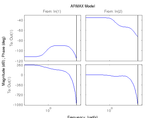
modelARMAX = armax(data,[na [nb nb] nc [nk nk]]);
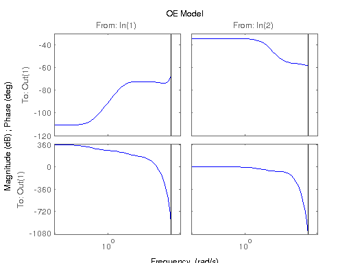
modelOE = oe(data, [[nb nb] [na na] [nk nk]]);
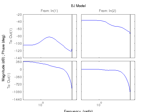
modelBJ = bj(data, [[nb nb] nc nd [na na] [nk nk]]);
Time domain data set with 72901 samples.
Sampling interval: 0.001

Outputs      Unit (if specified)
   y1

Inputs       Unit (if specified)
   u1
   u2
Convert to statespace and returns a decomposition of the model into the observable and unobservable subspaces.
a = idss(modelARX);
[A,B,C,T,k] = obsvf(a.A,a.B,a.C);
sys = ss(A,B,C,a.D,modelARX.Ts);

a = idss(modelARX3);
[A,B,C,T,k] = obsvf(a.A,a.B,a.C);
sysARX3 = ss(A,B,C,a.D,modelARX3.Ts);

a = idss(modelARMAX);
[A,B,C,T,k] = obsvf(a.A,a.B,a.C);
sysARMAX = ss(A,B,C,a.D,modelARMAX.Ts);

a = idss(modelOE);
[A,B,C,T,k] = obsvf(a.A,a.B,a.C);
sysOE = ss(A,B,C,a.D,modelOE.Ts);

a = idss(modelBJ);
[A,B,C,T,k] = obsvf(a.A,a.B,a.C);
sysBJ = ss(A,B,C,a.D,modelBJ.Ts);
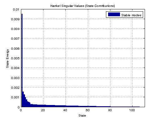
Order Reduction
Computes the Hankel singular values hsv of the dynamic system sys. In state coordinates that equalize the input-to-state and state-to-output energy transfers, the Hankel singular values measure the contribution of each state to the input/output behavior. Hankel singular values are to model order what singular values are to matrix rank.
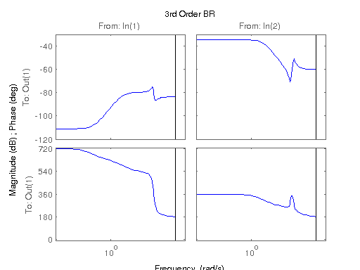
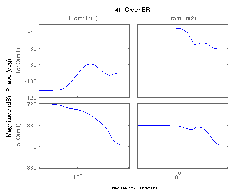
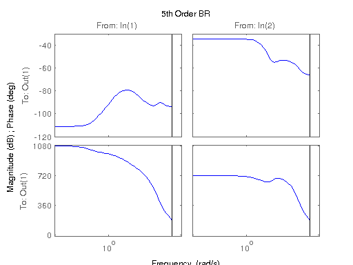
We then use balred to reduce the model order through use of a balanced realization.
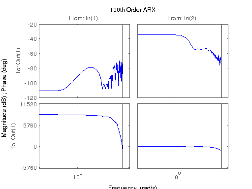
figure;
hsvd(sys); % Check out what orders contain the most amount of energy.
sys3 = balred(sys, 3)
sys4 = balred(sys, 4)
sys5 = balred(sys, 5)

figure;
bode(sys3);
title('3rd Order BR');
figure;
bode(sys4);
title('4th Order BR');
figure;
bode(sys5);
title('5th Order BR');
figure;
bode(sys);
title('100th Order ARX');
figure;
bode(sysARX3);
title('3rd Oder ARX');
figure;
bode(sysOE);
title('OE Model');
figure;
bode(sysBJ);
title('BJ Model');
figure;
bode(sysARMAX);
title('ARMAX Model');
a =
             x1        x2        x3
   x1     0.953    0.2052   0.01946
   x2  -0.09065     1.098    0.2412
   x3   0.06411   -0.1237    0.8559

b =
               u1          u2
   x1  -1.856e-06   -0.002165
   x2   0.0001254   0.0001829
   x3  -7.085e-05   0.0002413

c =
             x1        x2        x3
   y1   -0.1186  -0.01792   -0.1334

d =
               u1          u2
   y1  -6.173e-05  -0.0008695

Sampling time (seconds): 0.001
Discrete-time state-space model.

a =
              x1         x2         x3         x4
   x1     0.7566    -0.1398     0.5856    -0.2578
   x2     0.2515     0.9966    -0.1714     0.1034
   x3     0.0448    0.06568     0.7407     0.1338
   x4  -0.007778   -0.01769    0.06589     0.9607

b =
               u1          u2
   x1  -0.0001264   -0.005856
   x2    4.28e-05   0.0006873
   x3   6.846e-05    0.002724
   x4  -2.002e-05    -0.00096

c =
            x1       x2       x3       x4
   y1  0.04525  -0.1192  -0.1168  0.01011

d =
              u1         u2
   y1  1.887e-05  0.0004616

Sampling time (seconds): 0.001
Discrete-time state-space model.

a =
               x1          x2          x3          x4          x5
   x1      0.6903     -0.5091     -0.3041      0.4811     -0.1035
   x2      0.1544      0.7294     -0.1825      0.8653  -0.0009059
   x3      0.2542      0.1104       1.092     -0.2477     0.06413
   x4    -0.05073     0.06509     0.07993      0.4394    -0.03276
   x5     0.02531     -0.1257     -0.0902      0.3841      0.9944

b =
               u1          u2
   x1  -7.601e-05   0.0007801
   x2  -0.0001636   -0.004855
   x3   3.768e-05    0.001123
   x4   0.0001206    0.003997
   x5  -7.311e-05   -0.001823

c =
             x1        x2        x3        x4        x5
   y1  -0.04945  -0.03785    0.1087    0.0277    0.0246

d =
               u1          u2
   y1  -4.194e-06  -0.0001146

Sampling time (seconds): 0.001
Discrete-time state-space model.
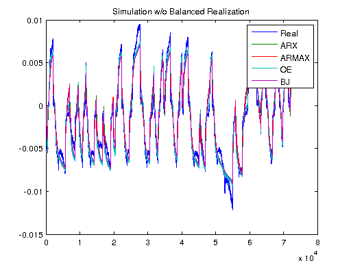
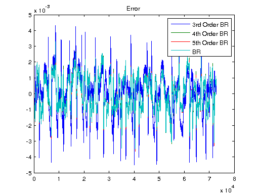
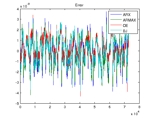
Simulation Of Models To Real Data
Using lsim to look at the differences between the actual data, and what our models will predict the output to be.
Ts = 1/1000;

V = [U1, U];
T = Ts*(0:length(V)-1);

y3 = lsim(sys3, V);
y4 = lsim(sys4, V);
y5 = lsim(sys5, V);
ysys = lsim(sys, V);
yARX3 = lsim(sysARX3, V);
yARMAX = lsim(sysARMAX, V);
yOE = lsim(sysOE, V);
yBJ = lsim(sysBJ, V);

figure
plot([Y y3 y4 y5 ysys])
legend('Real','3rd Order BR','4th Order BR','5th Order BR', 'BR');
title('Simulation of Order-Reduction and Balanced Realization');

plot([Y yARX3 yARMAX yOE yBJ])
legend('Real','ARX','ARMAX','OE', 'BJ');
title('Simulation w/o Balanced Realization');

figure
plot([Y-y3 Y-y4 Y-y5 Y-ysys])
title('Error');
legend('3rd Order BR','4th Order BR','5th Order BR', 'BR');

figure
plot([Y-yARX3 Y-yARMAX Y-yOE Y-yBJ])
title('Error');
legend('ARX','ARMAX','OE', 'BJ');
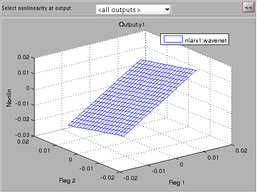
Non-Linear Model
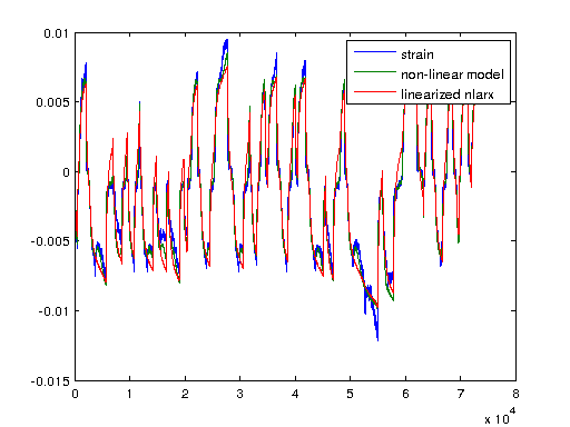
I'm plotting a non-linear ARX model of the system here with 5 regressors and a wavelet network with 57 units which was modeled to the same iddata object. First we'll look at the non-linearity of the wavenet and then simulate the output strain with both the non-linear model and a linearized verion of the nonlinear autoregressive approximation using linapp. Linapp does /not/ use a tangent linearization approach and should work better for larger ranges of input 'u'.
figure;
plot(nlarx1);
figure;
a = linapp(nlarx1,V);
a = idss(a);
a = ss(a.A, a.B, a.C, a.D, 1/1000);
plot([Y sim(nlarx1, V) lsim(a, V)]);
legend('strain', 'non-linear model', 'linearized nlarx');